 Protein Structure BasicsProtein Structure Basics
Proteins are macromolecules (heteropolymers) made up from 20 different L-a-amino acids, also referred to as residues. Below about 40 residues the term peptide is frequently used. A certain number of residues is necessary to perform a particular biochemical function, and around 40-50 residues appears to be the lower limit for a functional domain size. Protein sizes range from this lower limit to several hundred residues in multi-functional proteins. Very large aggregates can be formed from protein subunits, for example many thousand actin molecules assemble into a an actin filament. Large protein complexes with RNA are found in the ribosome particles, which are in fact 'ribozymes'.
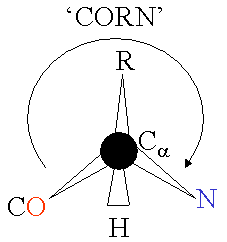
The basic structure of an a-amino acid is quite simple. R denotes any one of the 20 possible side chains (see table below). We notice that the Ca-atom has 4 different ligands (the H is omitted in the drawing) and is thus chiral. An easy trick to remember the correct L-form is the CORN-rule: when the Ca-atom is viewed with the H in front, the residues read "CO-R-N" in a clockwise direction.
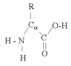
The different side chains R determine the chemical properties of the amino acid or residue (the residue is the amino acid side chain plus the peptide backbone, see below).
| Name (Residue) | 3-letter code | Single code | Relative abundance (%) E.C. |
MW | pK | VdW volume(Ĺ3) | Charged, Polar, Hydrophobic |
| Alanine | ALA | A | 13.0 | 71 | 67 | H | |
| Arginine | ARG | R | 5.3 | 157 | 12.5 | 148 | C+ |
| Asparagine | ASN | N | 9.9 | 114 | 96 | P | |
| Aspartate | ASP | D | 9.9 | 114 | 3.9 | 91 | C- |
| Cysteine | CYS | C | 1.8 | 103 | 86 | P | |
| Glutamate | GLU | E | 10.8 | 128 | 4.3 | 109 | C- |
| Glutamine | GLN | Q | 10.8 | 128 | 114 | P | |
| Glycine | GLY | G | 7.8 | 57 | 48 | - | |
| Histidine | HIS | H | 0.7 | 137 | 6.0 | 118 | P,C+ |
| Isoleucine | ILE | I | 4.4 | 113 | 124 | H | |
| Leucine | LEU | L | 7.8 | 113 | 124 | H | |
| Lysine | LYS | K | 7.0 | 129 | 10.5 | 135 | C+ |
| Methionine | MET | M | 3.8 | 131 | 124 | H | |
| Phenylalanine | PHE | F | 3.3 | 147 | 135 | H | |
| Proline | PRO | P | 4.6 | 97 | 90 | H | |
| Serine | SER | S | 6.0 | 87 | 73 | P | |
| Threonine | THR | T | 4.6 | 101 | 93 | P | |
| Tryptophan | TRP | W | 1.0 | 186 | 163 | P | |
| Tyrosine | TYR | Y | 2.2 | 163 | 10.1 | 141 | P |
| Valine | VAL | V | 6.0 | 99 | 105 | H |
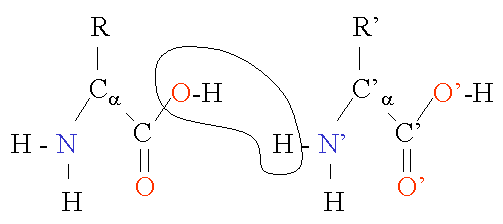
Two amino acids are combined in a condensation reaction. Notice that the peptide bond is in fact planar due to the delocalization of the electrons. The sequence of the different amino acids is considered the primary structure of the peptide or protein. Counting of residues always starts at the N-terminal end (NH2-group).
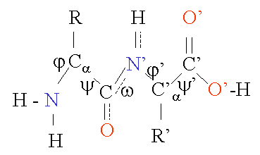
In contrast to the rather rigid peptide bond angle w (always close to 180 deg) , the bond angles phi j and psi f can have a certain range of possible values. They are restrained by geometry to allowed ranges typical for particular secondary structure elements, and represented in a Ramachandran plot (discussed below). A few important bond lengths [1] are given in the table below.
| Peptide bond | Average length | Single Bond | Average length | Hydrogen Bond | Average (±0.3) |
| Ca - C | 1.53 (Ĺ) | C - C | 1.54 (Ĺ) | O-H --- O-H | 2.8 (Ĺ) |
| C - N | 1.33 (Ĺ) | C - N | 1.48 (Ĺ) | N-H --- O=C | 2.9 (Ĺ) |
| N - Ca | 1.46 (Ĺ) | C - O | 1.43 (Ĺ) | O-H --- O=C | 2.8 (Ĺ) |
The polypeptide chain of a protein seldom forms just a random coil. Remember that proteins have either a chemical (enzymes) or structural function to fulfill. High specificity requires an intricate arrangement of 3-dimensional interactions and therefore a defined conformation of the polypeptide chain. In fact, some neurodegenerative diseases like Huntington's may be related to random coil formation in certain proteins. The two most common secondary structure arrangements are the right-handed a-helix and the b-sheet, which can be connected into a larger tertiary structure (or fold) by turns and loops of a variety of types. These two secondary structure elements satisfy a strong hydrogen bond network within the geometric constraints of the bond angles w, j and f . The b-sheets can be formed by parallel or, most common, antiparallel arrangement of individual b-strands.
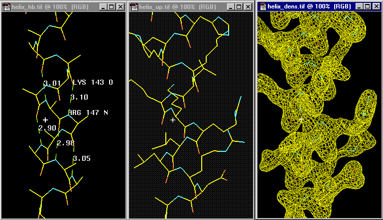
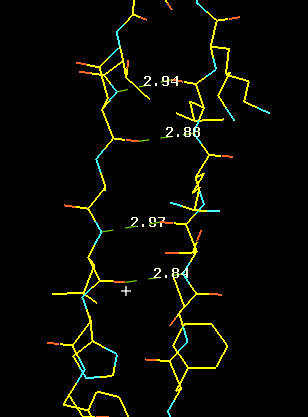
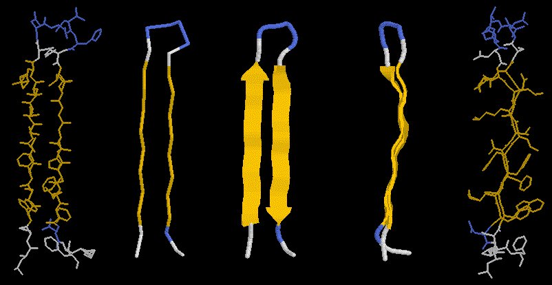
The left panel shows the hydrogen bonding in an actual a-helix backbone. Note that the n th residue O (Lys 153) bonds to the n+4 th following residue's N (Arg 147). The actual values of some displayed H-bond distances give you some idea about the variations to expect within a helix. The center panel includes the side chains which were omitted in the left panel for clarity. You see the side chains pointing towards the N-terminal of the chain (lower residue numbers) and thus it is usually possible to determine the direction of the helix quite well during initial model building. A very nice 2Ĺ electron density is shown in the right panel.
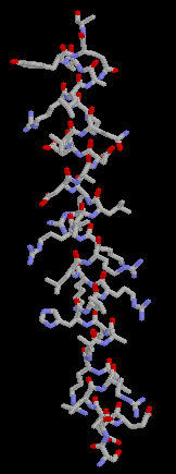
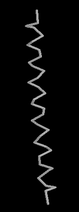
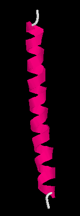
Here are some more representation of the same helix, ball and stick,
backbone and the secondary structure cartoon (linguini diagram).
Quiz : where is the N-termial of this helix?
Top or bottom of the figures?
Here we see the hydrogen bond network in a 2-stranded, antiparallel b-sheet. The side chains are sticking out avove or below the plane of the picture. It less clear cut than in the case of the helix, in which direction to initially trace a beta sheet strand. The beta sheet can be infinitely extended due to the repeatable H-bonding pattern to either side of a strand. Look at our pdb entry 1JBC or 1E01or a nice example of a beta sandwich.
The pleated nature of the sheet becomes distinctly visible in the righ panels of this figure, showing also the side chains sticking out above and below the sheet plane. If you look carefully, you will also notice that the sheet has a left twist (centre panel).
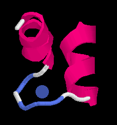
Turns, loops and a few other secondary structure elements such as a 3-10 helix complete the picture. We have now enough pieces to assemble a complete protein, displaying its typical tertiary structure. Look at our pdb entry 1bpi for a very simple, 58-residue protein containing 2 strands and 2 short helices. For information on the function of recognition loops, see our antibody work.
Despite that there are about 100,000 different proteins expressed in eukariotic systems, there are much fewer different structural motifs and folds, partly as a consequence of evolved pathways and mechansims. Motif in this sense does refer to a small specific combination of secondary structure elements (such as helix-turn-helix), and not to the contents of the asymmetric unit cell as used as a crystallographic term. Fold referes to a global type of arrangement, like helix-bundle or b-barrel. Many good textbooks [2,3] describe folds and motifs, so we will limit ourselves to those where we have examples on our site.
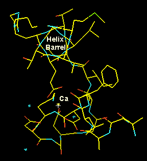
A typical small motif is the calcium binding EF-hand in calmodulin, a ubiquitions molecule undergoing Ca-dependent conformational changes. It contains 4 Ca++ ions which are coordinated in a typical fashion in a helix-turn-helix motif called the EF-hand:
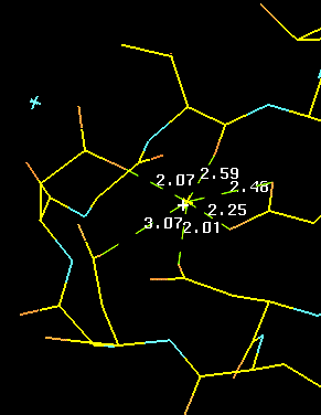
The positively calcium atom Ca++ iis coordinated through hydrogen bonds with acidic (negatively charged) aspatrate and glutamate residues as well as with backbone oxygen atoms (Left, below). In the right panel we look down the barrel of one of the helices towards the CA in the loop. Note the typical pattern (well-known to model builders) displaying the chatacteristic staggering pattern with the hole in the centre of the helix.
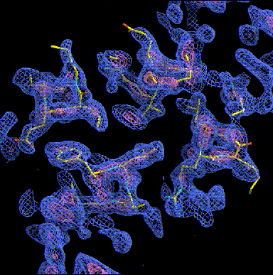
Other typical motif in the apha-domain structures is the 4-helix bundle. Ferritin (see our Cd-crystallizaion paper), Cytochtome b562, or apo-E are typical examples. The helices are amphipatic (hydrophobic residues on one side, charged ones on the other and pack antiparallel with the hydrophobic sides towards each other forming a hydrophobic core. In the following we look down the helices (note the holes in the helix core) in a 2Ĺ experimental MAD map. Note the hydrophobic residues packed insde and the charged ones at the outside of the helices. The picture gives you also a good idea what the crystallographer actually sees whe he starts model building.
References
[1] Engh R A & Huber R (1991). Accurate bond and
angle parameters for X-ray protein structure refinement. Acta Cryst., A47, 392-400.
[2] Branden C & Tooze J (1991). Introduction to Protein Structure.
Garland Publishing inc, New York and London.
[3] Alberts B, Bray D, Lewis J, RAff M, Roberts K, Watson JD (1994).
Garland Publishing inc, New York and London.
![]() Back to X-ray Tutorial Introduction
Back to X-ray Tutorial Introduction
LLNL Disclaimer
This World Wide Web site conceived and maintained by
Bernhard Rupp (br@llnl.gov)
Last revised August 09, 2000 12:31
UCRL-MI-125269