|
News Introduction Screenshots Download Installation License |
|
|
|
Examples Tutorial PbSO4 Tutorial Cimetidine F.A.Q. Hints & tricks |
|
|
|
Archive |
|
|
|
SF project page Browse CVS |
Command-Line options
It is possible to use command-line arguments for Fox (use
Fox -h to get all options), e.g.: "Fox -i silicon.xml"will load the silicon.xml file and launch the GUI."Fox -i silicon.xml --nogui -n 10000 -o out.xml"will load the silicon.xml file, and run the optimization without GUI for 10000 trials, then output to out.xml."Fox -i example/pbso4-joint.xml --nogui --randomize -n 100000 --finalcost 1000 -o test.xml"will run Fox (without GUI) on the PbSO4 example for at most 100000 trials after first randomizing the structure (useful for tests), and stop the optimization when the overall cost falls below 1000, then output the result to test.xml . You can run that one from the main Fox directory."Fox -i alumina.xml --loadfouriergrd alumina.grd"will load the alumina.xml file, and display the first crystal structure in 3D, and load the fourier map as well. The.grdfourier map can be generated by expgui, gsas, and theforgridpackage which you can get from ftp://ftp.ncnr.nist.gov/pub/cryst/gsas/ (precompiled binaries in the exe_{linux|sgi|win} directories)."Fox -i alumina.xml --loadfourierdsn6 alumina.DN6"will load a DSN6 fourier map and display it with the first crystal structure in the xml file. The DSN6 fourier map can be created using the 'O' command in GSASforplot("Convert map to DSN6 format"). You must use a z-sliced fourier map, and the fourier map must go from 0.0 to 1.0 along all 3 directions, as Fox does not take care of filling the remaining of the Fourier map by symmetry."Fox --speedtest"Do a speedtest of Fox (takes about 1mn30s).
Reference Manual
Note About Parameters
- All the parameters that can be optimized in Fox have two checkboxes between the name and the field where you can read and enter the value for the parameter. The left checkbox (R) can trigger the "refinable" status of the parameter (unchecked= not optimized), and the right one (L) enables the limits for that parameter.
- For some parameters (e.g. the atoms positions in a Molecule), you may not have access to these fix/limit buttons, because the functionnality to restrain the evolution parameters is provided at a higher level (e.g. in the Molecule object, atoms positions are limited relatively to each other through intelligent restraints, not individual limits).
- Also, some parameters who do have R/L checkboxes cannot be optimized by Fox, because it does not make sense to refine some parameters using a global optimization algorithms. See the FAQ
for a few more details.
Main Menus
- The "File" menu allows to save or load a sort of "project" file in which are saved Crystal structures, diffraction data, algorithms... In fact everything which can be seen in the Fox main window is saved. It is saved in an XML format specific to Fox/ObjCryst++. You can also exit (but don't forget to save before, because Fox will not query you if you have not saved before !)The "Objects" menu can be used to create new Crystal, PowderPattern, DiffractionDataSingleCrystal and algorithms objects. Remember that you can create several of these objects simultaneously (limited only by scrollbar lengths!).
- The "Help" menu gives you access to the "about box" of Fox, and you can toggle the use of tooltips (which are not much used yet...).
Crystal Structure
(click on image to jump to the relevant section)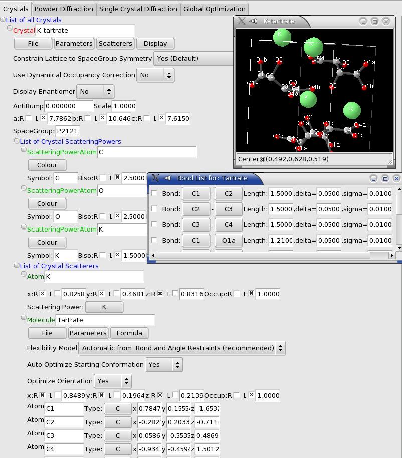
3D Crystal view
- You can open a 3D view (uses OpenGL) of the Crystal structure from the "Display" menu. You can then control the view with the mouse:
- Dragging with the left button will rotate the view, simulating a trackball.
- Shift-dragging with the left button will translate the center of the view (the coordinates in fractionnal coordinates are displayed at the bottom of the window).
- Dragging with the middle button: up/down will move the molecule closer or farther, and left/right dragging will change the perspective (increase or dercrease the angle view).
- A right-button click will pop-up a menu to allow you to:
- Toggle the display of the atom labels
- Change the display limits of the atoms (note: for Molecules, the limits apply to the center of the Molecule, so that the molecule is never cut)
- Toggle the display of the Crystal structure (useful if you are displaying a Fourier map)
- Import and control the display of Fourier maps: add or modify a contour value, change the color, toggle between wireframe and filled display style. To create Fourier maps using GSAS and EXPGUI, refer to the explanations in the command-line options.
- Export the view to a POV-Ray file so that you can create a ray-traced image of your structure (example on K-Tartrate). Atoms, Molecules and fourier maps are rendered. Atom labels and the deprecated ZScatterer are not exported. NOTE: if the image appears mirrored (left/right) in POV-Ray (seems to depend on POV-Ray version...), you can invert it by changing the
"right <-1.33,0,0>"statement in the "camera" section (near line 48) to"right <1.33,0,0>".
Crystal Menus
- "File" allows you to save all the atom positions and occupancies in a text file. The output also lists the interatomic distances to help deciding which atoms should be removed/merged. It is currently the only output possible (besides xml) of the crystal structure.
- "Parameters" allows you to:
- Add an antibump distance: you will be prompted to select the two atom types (scattering powers) between which you want to set up an antibump distance, and the corresponding distance.
- Note1: you can select the two identical atom types to declare, e.g., an O-O antibump. For same element antibump, the antibump penalty diminishes to 0 to enable merging of these atoms so that the dynamical occupancy correction can fully work; the antibump is then actually maximum at half the given the antibump distance.
- Note2: the antibump cost is displayed just above the Unit Cell parameters. It is multiplied by the "Scale" field beside. You may need to increase this scale factor if you want to give a larger weight to the antibump restraint, relatively to the diffraction data Chi^2. Alternatively, you can set the scale to zero to deactivate the use of the antibump (and thus compute faster).
- Fix or un-fix all parameters of the structure. Also see the FAQ "What parameters can/should I optimize".
- randomize the configuration. This does not affect fixed parameters, and takes into account the limits set for the parameters.
- Add an antibump distance: you will be prompted to select the two atom types (scattering powers) between which you want to set up an antibump distance, and the corresponding distance.
Crystal Options
- "Use Dynamical Occupancy Correction": this is an important feature of Fox: basically, you should use "yes" for inorganic compounds and "no" for organic ones. This allows to dynamically (without any a priori information or user intervention) take into account atoms on special positions and atoms shared between building blocks (one oxygen of a PO4 tetrahedron overlapped with another from a WO6 octahedron). The idea is to change the "dynamical" occupancy of the atoms during the calculations, so that if n atoms of the same type are overlapping, their occupancies are set to 1/n, and therefore they look like a single atom. This is transparent to the user, and you can know what the value of this "dynamical occupancy" is when saving the crystal structure in a text file.
- "Display Enantiomer": this can be used to display the enantiomeric structure in the 3D Crystal structure window, and can be useful to compare structures. It does not affect in any way the structural parameters, or the calculation of structure factors.
- "Constrain Lattice to SpaceGroup Symmetry": this option can be used to allow crystallographic symmetry not compatible with the unit cell (e.g. a cubic spacegroup and a tetragonal unit cell). This can be used for for phase transitions, to reduce the number of independent parameters, when you know (or can guess) a higher symmetry your structure is derived from.
Crystal Unit Cell & Spacegroup
- You can enter the spacegroup using either symbol or spacegroup number. The spacegroup field will revert to the previous entry if the value was not understood. In doubt (when not using a standard setting), you can use the full Hermann-Mauguin symbol (eg '-I 4bd 2c 3', 'P1121/a',...).
- The unit cell parameters can be entered in Angstroem and degrees. Only the relevant fields will be displayed after the spacegroup has been entered and processed (e.g. only the 'a' parameter for cubic spg). Note that the cell parameters cannot be optimized using the available algorithms.
Crystal Scattering Powers (atom types)
- For each element you want to use in your structure you must first declare the "atom type", which corresponds to the scattering factor (Thomson and resonant parts) and the temperature factor (currently only Biso is available). Normally, you will declare only one ScatteringPower by type of atom, unless you want, e.g., 2 oxygens with very different Biso. You can add (and remove) ScatteringPowers using the Crystal menu 'Scatterer'->'Add(Remove) ScatteringPower'.
- Note that you can also add a "spherical scattering power", which can be used to modelize a disordered fullerene. The total scattering power corresponds to only one electron, so that you must change the atom occupancy to correct that (e.g. for C60, use occupancy= 60*6 electrons). You will need to change the limits on the occupancy before doing that (right-click on the occupancy name, and change the default limits which are [0;1]).
- The name of the Scattering power is free format, but the symbol must correspond to one entry of the scattering factors tables in the international tables for Crystallography, i.e. the standard name for an atom or ion: 'C', 'O', 'Se', 'Cu2+',...
- You can change the colour displayed for each type of atom by using the 'Colour' menu and entering the RGB (red, green blue) components (all between 0.0 and 1.0).
- You can optimize the Biso value, although as long as you are far away from the good configuration it is a bad idea (useless, and slowing down a lot the algorithm). You should give approximate Biso values that you guess from other similar compounds. Since the algorithm is focused on low-angle, the sensitivity to Biso is fairly low.
Crystal Scatterers
The Scatterers in each Crystal structure can be either individual atoms or ZScatterers (molecules, polyhedra).
-
Atom:
This is the most basic Scatterer. You should try as much as possible to use large building blocks (see below the ZScatterer), since that will greatly reduce the number of parameters ( W+6O as atoms is 21 parameters, whereas a WO6 octahedron is 6 parameters).To add one atom, use the Crystal 'Scatterer'->'Add an Atom'. You will be prompted to choose the ScatteringPower for this atom from those that you have declared. You can fix /unfix all parameters (xyz, occupancy) through the GUI, as well as change the limits by right-clicking on the parameter's name.
-
Z-Scatterer(molecule, polyhedron):
Z-Scatterer are now obsolete. Although you can still read Fox xml files created with a z-matrix scatterer, you cannot create one any more. You should instead use a Molecule object, which is more flexible and gives much better results during global optimisations. If you want to re-use a given Z-Scatterer, you are strongly advised to convert it to a Molecule description, using the Import/export menu of the ZScatterer. It should add the missing bonds, as analyzed from bond distances. -
Molecule (organic compound, inorganic polyhedron):
A Molecule is defined by a list of atoms with their xyz coordinates (in an orthonormal reference frame internal to the molecule), with the geometry of the Molecule set by a list of restraints: bond lengths, bond angles and dihedral angles. The orientation of the Molecule is defined internally by a quaternion, so its parameters are not directly accessible.Note that to see the list of bonds, bond angles and dihedral angles you can use the menu "Formula->Show Bond List" etc...
To create Manually a Molecule, use first the Scatterer menu of the Crystal, and then using the menus of the Molecule Object, you can add all the atoms, and then all the restraints (bond lengths, angles, dihedral angles). A few notes when creating Molecules:
- Try to avoid dihedral angles as much as possible, as they tend to restrict a bit too much the movements of the Molecule during the global optimisation, and therefore hinder the progress towards the global minimum. Generally, several bond angles can replace very efficiently a dihedral angle.
- Two atoms are not required to be bonded to be used in a bond/dihedral angle restraint (although it generally is the case, but you may want to do strange things..)
- When you first add the atoms, they are all at (0,0,0) in the Molecule reference frame. You can use the menu to Optimize the initial conformation of the Molecule and see a more reasonable conformation, taking all restraints into account. If you do not do it, it will be automatically be done when you launch the global optimization.
There are several levels of flexibility available for a Molecule:- "Automatic from Bond and Angle restraints": this is the default choice. In this mode, Fox will allow atoms to move slightly away from the 'ideal' positions defined by the length and angular restraints. This is useful when you do not know exactly the bond lengths or angles. It can also be useful when you know them, as the additional flexibility will 'smooth out' the Chi^2 hypersurface, and therefore improve the convergence of the algorithm. Fox will automatically detect free torsion bonds (those not involved in a cycle or with a dihedral angle restraint).
- Details on the calculations of restraints can be found by opening the 'bond', 'bond angle' and 'dihedral angle' windows. These include the expected (ideal) value, as well as the 'delta' and 'sigma' parameters.
- The restraint cost for bond lengths, bond angles and dihedral angles is calculated using two parameters delta and sigma for each restraint. e.g. for a bond of expected value d0, if the calculated value is within [d0-delta;d0+delta], there is no restraint cost. Out of this range the restraint is equal to [d-(d0+delta)]^2/sigma^2 (above d0+delta), and [(d0-delta)-d]^2/sigma^2 (below d0-delta). The sigma (resp. delta) parameter is by default equal to 0.01 (resp. 0.02), in Angstroems or radians. Fox has been optimized with these default values and it is highly recommended not to change them. If you feel you know what you are doing, you can do it in the bond, bond angles and dihedral angles windows, which can be accessed through the "formula" menu.
- "Rigid Body": in this mode the geometry is rigorously fixed, only the orientation is optimized unless the "Optimize Orientation" option is set to "No".
- "User-Chose Free Torsion": in this mode you can select which bonds are free rotors in the Molecule (open the Bond list from the "formula" menu and use the left checkbox to mark the free torsions).
- "Auto Optimize Starting Conformation": this is only needed if the initial conformation of the Molecule does not respect the restraints, e.g. if you added manually a few restraints or if you added all atoms by hand rather than using a z-matrix import.
This will trigger an optimization of the conformation at the beginning of a global optimization. The option will self-deactivate itself as soon as it is done. - "Optimize Orientation": whether or not to optimize the orientation of the Molecule. This is only meaningful if you are using the "Rigid Body" mode for flexibility. Note that as the orientation is parametrized using quaternions, the orientation parameters are not accessible as the usual phi-chi-psi angles.
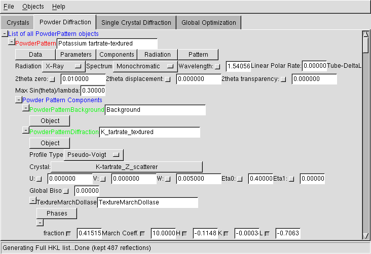
Powder Pattern
Powder Menus
- "Data" allows to import several types of data. If you wish to add another format, send an email to me with an example data, and saying why you think it is important that this format is supported. You can also save the calculated and observed spectra, and use the 'simulation mode', which will use a dummy observed pattern (I=1. in all points).
- "Parameters" allows you to fix all parameters. Note that only preferred orientation parameters and the global temperature factor are refinable anyway.
- "Components" is the menu to describe your powder pattern in terms of the sum of components, which can be one interpolated background, and any number of crystalline phases.
- "Radiation" allows you to choose the radiation for your experiment. It is also possible to use the radiation interface just below the menus, but to choose an X-Ray tube it is easier that way (unless you know by heart the delta-lambda !). Do not forget to input the correct polarization rate (0.95 typically for a synchrotron experiment).
- "Pattern" allows you to open the graph window with the observed and calculated patterns, and to fit the scale factor. It is also possible to add "excluded 2-theta zones" which will be ignored during global optimization: you will be prompted for the minimum and maximum 2theta values of the region to ignore (to remove those regions, you have to edit the xml file).
Radiation
Here you can describe the radiation corresponding to your experiment (neutron, X-Ray, tube,...). The wavelength is in Angstroem as usual. Set the polarization rate between 0.95 and 1 for synchrotron experiments, and 0 for an X-Ray tube (actually if you use a monochromator it should be above 0, but a precise value is not critical for a global optimization).2theta correction parameters
These parameters allow to correct for experimental errors in the 2theta positions of reflections, due to a wrong zero, or a misplacement of the sample holder or its transparency. Practically, using the 2theta zero is sufficient (note that it does not necessary correspond to the convention used by other programs, you may have to change the sign and/or to multiply by 2 the value). After each change, you can right-click on the powder pattern graph to update it.Maximum sin(theta)/lambda
Use this field to limit the extent of the calculations on the powder pattern. It is usually a very good idea to do that, since for a global optimization, high-angle data is useless. A good value is 0.25 Angstroem-1 (corresponding to a resolution of 2 Angstroems), although you can go higher to 0.4 A-1 if you feel there are not enough reflections...Powder Pattern Background
So far the background can only modelized using linear interpolation between at user-chosen 2theta values. To input the (2theta, intensity) points you must create a text file with a list of "2theta intensity" on each line (2theta in degrees), and load it using the menu. See the tutorials for examples.If you want to change the points, just change the values in the text file, and reload it from the menu.
There is currently no limit to the number of points, but even for complex backgrounds 10 should be enough.
PowderPatternDiffraction: Crystalline contribution to the powder pattern
This allows to describe the contribution of a crystalline phase to the powder pattern. It is possible to save the calculated structure factors using the menu (note that structure factors above the chosen sin(theta)/lambda limit are not calculated).
Profile parameters
These are the usual profile parameters:- A pull-down menu allows you to xhoose between Gaussian, Lorentzian and pseudo-Voigt.
- U V W defining the width using Caglioti's law (W is the constant width, which is generally sufficient if you are using integrated Rfactors as recommended)
- Eta0 (constant) and Eta1 (theta-dependant) define the mixing parameter for a pseudo-Voigt profile.
Crystal choice
You are asked to choose a crystal structure upon creation of the PowderPatternDiffraction object. You can change it afterwards by clicking on the crystal name.Global Biso
This can be used as a global temperature factor for this crystalline phase (affects all atoms). This is refinable, although it slows the optimization without helping a lot.Texture (Preferred Orientation) using the March-Dollase Model
FOX supports optimization of Preferred orientation, usign the March-Dollase model. To add one phase, use the "Phases" local menu. You can then enter the fraction, March coefficient (>1 for needles, <1 for plate-like crystallites), and HKL coordinates for the preferred orientation.Note: it is very important to use this only as a last resort, or if you know for sure that you have preferred orientation. Taking one more day to prepare carefully a non-textured sample is definitely worth it, since even if a solution is found, it will be much slower - preferred orientation reduces the information available in some direction of the crystal.
If you finally decide to search for preferred orientation parameters, it is recommended to input as much information as possible. For example, you should be able to know what kind of preferred orientation to expect (plates or needles), so that you can restrict the March coefficient to be either >1 or <1 (e.g. use limits [.1;1] or [1;10] - never go below .1 or above 10, that would just slow things). If you know what the preferred orientation vector is, that's even better.
Note that it is possible to use several preferred orientations, but I strongly discourage to do this for a global optimization.
Single Crystal Diffraction Data
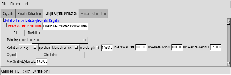
Note that the support for single crystal data is very limited, as generally direct methods will do a quick job out of any good single crystal data. This is nevertheless provided, since in some cases the robustness of direct-space methods can make a difference. The 'intensities' which are to be imported into Fox must be fully corrected (absorption & Lorentz-Polarization), so that you actually need |F(hkl)|^2.
Menus
You can use the menus to load data from a text file (either four columns H K L Iobs, or five columns H K L Iobs sigma). If you do not have data, you can also use the "simulation mode" and generate a full list of H K L up to a given 2theta value. Finally, you can export the structure factors in a text file.Twinning option
This is a "trick" to have a very basic handling of twinned single crystal data. If selected, comparison between observed and calculated intensities will not be made on individual reflections, but on the sum of intensities of reflections with approximately identical 2theta angle (i.e. not only equivalent reflections). This allows to search for a crystal structure without any knowledge on the type of twinning, effectively handling the data as "powder data", but without any computing penalty.Radiation
Same as for powder pattern...Crystal
You can click on the crystal name to change the crystal structure associated to this data.Maximum sin(theta)/lambda
Same as for powder pattern...Global Optimization Algorithms
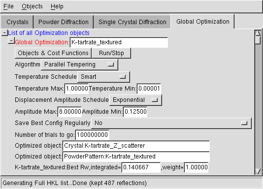
Menus
- Use the "Objects" to define the objects that you want to use (i.e. the crystal structure and the associated diffraction dataset(s) ).
- Use the "Run/Stop" to launch and thereafter to stop the optimization.
Algorithm
You can choose between Parallel Tempering (highly recommended) and Simulated Annealing (use this only if you know how... you'd have to carefully choose the number of trials). Normally, the default choice (Parallel Tempering) should not be changed.Temperature
These are the minimum and maximum temperatures to ensure that the algorithm will search all possible configurations, while insisting on the best configurations. It is highly recommended not to change the default choices, with a "smart" temperature schedule which will be tuned by the algorithm.Displacement amplitude
These are used to define the amplitude of displacements of all parameters during random moves. Again, you should not change the default parameters which should be fine for any optimization, with an exponential schedule.Autosave
This allows you to save regularly the "best" configuration reached by Fox. Note that the saved xml files will always be in the working directory (i.e. the one from which you launched FOX, or the directory of the FOX application).Trial
Put here the total number of trials that you want to make. For Parallel tempering, you can put a large number (100 000 000), and then stop manually the algorithm (using the "Run/Stop" menu) when it seems to have converged (the algorithm has the advantage of being invariant with the number of trials). (for simulated annealing, you need to more carefully evaluate the number of trials for your specific configuration...).Objects
This is the list of the objects to be optimized, which have been added through the menu.