TABLE OF CONTENTS

1. Introduction
2. System Requirements
3. User Instructions

• 3.1 Basic XFIT Operation
• 3.2 Saving XRD files
• 3.3 The Edit File Details Window
  • 3.3.1 Selecting More than One Item at a Time
• 3.4 Brief Instant Fitting Tutorials
• 3.5 Stripping ka2 from a Diffraction Line

• 4.1 Overview of Data Structures and Parameter Types
• 4.2 Summary of Fundamental Parameters Approach
• 4.3 Peak Types 114.4 Generation of a Peak
• 4.5 Preliminary to Refinement
• 4.6 Parameter Types and Aberration Functions
  • 4.6.1 The Convolution Step Parameter
• 4.7 Parameter Attributes
• 4.8 Calculating Peak 2thi Limits

1. Introduction

An interactive and graphical X-ray line profile fitting program XFIT has been developed for the MS Windows operating system. XFIT is a user friendly system written in the c++ programming language. It integrates the familiar Pseudo Voigt (PV) and Split Pearson (PVII) functions with a Fundamental Parameters (FP) convolution approach [2] [3] [4] to generating line profiles. This integration of profile generation strategies allows a calculated X-ray diffraction pattern (XRD) to be synthesised from any number of peaks of any type, with each peak consisting of an emission profile (LAM). For example, a peak could be generated using an emission profile consisting of two PVII LAM lines for ka1 and ka2 and then numerically convoluted with a Gaussian function to represent strain broadening, a Lorentzian to represent crystallite size broadening, or both a Gaussian and Lorentzian simultaneously.

1. System Requirements

The system requirements for XFIT are as follows:

Operating System : MS Windows and Win32s

Hardware : PC386 or higher.

Minimum 2M bytes of memory.

1. User Instructions

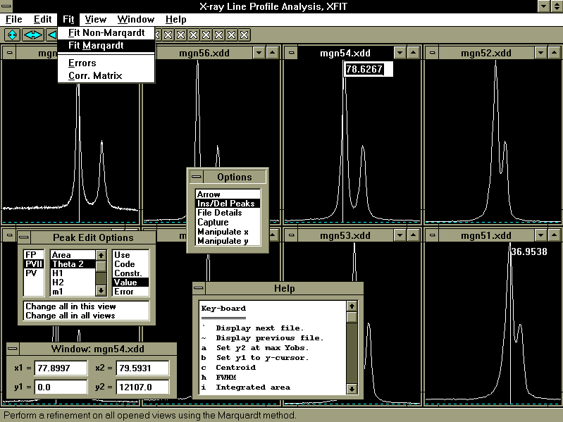
XFIT utilises the capabilities of the Multiple Document Interface (MDI) implementation of Borland c++ under MS Windows. MDI offers a flexible environment where any number of XRD files can be viewed in any number of graphics windows. More than one XRD file can also be displayed in the same window. Numerous other window types are available at the user's request; some of these are shown in figure 1 and descriptions given in table 1.

XFIT is primarily designed for accurate line profile analysis. It implicitly corrects Bragg 2q positions through the use of FP peaks, and it can give precise peak broadening characteristics. XFIT also offers excellent graphics facilities for displaying XRD data (see Appendix 3 for file types and formats).

WindowType	Purpose
Options	Edit/Show Options, A small window of frequently used options that is displayed on program execution.
Help	Help/Help, Displays the contents of the text file HLP.CPP in a text window. HLP.CPP contains a number of key-board commands that facilitate program operation.
Text	A text window is created when a text file is loaded. XFIT also generates a text window for the option Fit/Corr. Matrix.
Peak Edit Options	LMB on Ins/Del Peaks in Options window displays the Peak Edit Options window. This wondow allows the user to change peak parameters in a graphical manner.
Edit File Details	A window that is the main interface between the user and the data stored by XFIT.
Edit x-y scales	A means of numerically changing the x-y limits of a window.
Temporary Output	A small text window displayed by XFIT for temporary output.

Table 1 Window types available to the user. LMB and RMB corresponds to the pressing of the left and right mouse buttons. Underlined words/phrases corresponds to the selection of menu options. For example, File/Load Data means execute the File menu and then the Load Data option of the File menu.

Figure 1. Monochrome display of XFIT. XFIT is actually displayed in colour.

1. Basic XFIT Operation

Descriptions of the Options window and of the main menu options across the top of the screen (see figure 1) are given in tables 2 and 3. Windows can be opened and closed at any time at the users request. In some instances XFIT automatically closes windows to prevent clutter.

The x-y limits of the graphics windows can be changed using the three manipulation icons at the top left hand corner of the screen. These provide for most of the required manipulations as follows:

1st icon	LMB increases y2, RMB decreases y1.
2nd icon	LMB decreases x1, RMB increases x2.
3rd icon	LMB decreases x1 & x2 in equal amounts. RMB increases x1 & x2 in equal amounts.

Key-board manipulation instructions, given in the Help window, are often quicker and simple to use in this context..

The typical course of events during the operation of XFIT are as follows:

Load and display the required XRD files.

Assign an emission profile to each XRD file.

Insert peak positions using the Ins/Del Peaks option of the Options window by pressing the LMB. The RMB deletes the nearest peak to the mouse.

Execute Fit/Fit Marquardt to start a refinement.

Options Window
Arrow	Show the standard mouse cursor. In this mode the x-axis limits of the active graphics window can be changed using the LMB and RMB. The LMB pressed changes the x1 limit to the x-axis position of the mouse. The RMB pressed changes the x2 limit to the x-axis position of the mouse.
Ins/Del Peaks	Insert/delete peaks. Peaks are inserted at the position of the mouse using the LMB. The nearest peak to the mouse is deleted using the RMB.
File Details	Displays the Edit File Details window.
Capture	Changes the mouse cursor to capture mode. This mode allows a new XRD file to be created (Captured) from the displayed part of an XRD file. This is done by pointing to the desired XRD file and then pressing the LMB.
Manipulate x Manipulate y	These options changes the mouse cursor to manipulate mode. This mode allows manipulation of the actual data of displayed XRD files. Point and drag using the LMB/RMB to operate on the desired XRD file. The LMB performs translation. For Manipulate x, the RMB contracts/expands the x-axis limits of the XRD file. For Manipulate y, the RMB multiplies the XRD data.

Table 2 Description of the Options window operations.

File
Load Data Unload Data	Load/Unload XRD data, up to 32 graphics files can be loaded. Each loaded graphics file has a tick/cross icon assigned to it; this corresponds to display/hide the data respectively. Each graphics view displays its own set of ticks/crosses. More than one file can be loaded/unloaded at a time as describe in section 3.3.1.
New TXT Load TXT Save TXT Save TXT As	Text window file operations. The MS Windows text editing key-strokes are available for editing.
Load Project Save Project	Load/Save all data stored by XFIT into a project file (*.PRJ). Project files can be reloaded at a later time.
Exit	End XFIT. The user is prompted to save modified files.
Edit
Show Options	Display the Options window. This window is typically left displayed since it contains often used commands.
Edit x-y Scales	Edit the x-y limits of the graphics windows.
Create x-y Report	Save a text column report of the displayed graphics data of the active window. These reports can then be easily read by a spread sheet.
Fit
Fit Non-Marqardt Fit Marqardt	Start the refinement procedure. All displayed XRD data of the opened graphics windows are included in the refinement. If a graphics window is maximised then only its displayed XRD data are included in the refinement procedure. During refinement XFIT displays the calculated profile together with the observed profile at the end of each iteration.
Errors Corr. Matrix	Calculate the Errors/Corr. Matrix for the parameters associated with the displayed XRD data of the opened graphics windows. On calculation, the Corr. Matrix is displayed in a text window.
View
Show all of selected files	Displays in the active window all of the selected files (ticks).
Fix y2 at max y Fix y1 at min y	Fix the y2 (or y1) limit of the active window (or all windows) to the maximum (or minimum) y value of the displayed XRD data.
Fix y1 to zero	Fix the y1 limit of the active window (or all windows) to zero.
Cnts/Sec	Change the display of the displayed XRD data to Counts/Second.
Same x all views	Constrains the x-axis limits of all views to the active view.
Window
Cascade Tile Vertical Tile Horizontal Arrange Icons	Standard window manipulation operations.
Add View	Creates and displays a new graphics window.
View all files	Creates and displays a graphics window for each loaded XRD file.
View selected files	Creates and displays a graphics window for each selected (ticks) XRD file.
Help
Help	Displays a text window containing useful information on XFIT's operation.
About	XFIT Authors.

Table 3 Main menu and description of menu options.

1. Saving XRD files

XFIT prompts the user to save modified XRD files on program termination. Files are flagged as modified when they have been manipulated or Captured (see table 1 for descriptions of the Manipulate-x, Manipulate-y and Capture options of the Options Window). XRD files can also be saved or unloaded by pressing the RMB on the ticks/crosses (see top of screen in figure 1) which brings displays a pop-up menu with the following options:

Show all of this file

Unload

Save As

All files are saved in the XDD format as described in Appendix 3.

1. The Edit File Details Window

This window provides the interface between the user and the data stored by XFIT. Referring to figure 2, the operation of the Edit File Details window is simple and flexible and is as follows:

To change data, for example the H1 Value attribute of PVII peaks:

1. Locate the parameters using the LMB on the top left list box to expand/collapse headings.

2. Select the H1 values to be changed using the LMB. The H1 values can be selected in any order by holding down the Ctrl key. The whole H1 column can be selected by pressing the LMB on the H1 heading.

3. Type the new value at the Change Selections To position and press return to send this new value to the selected H1 positions. Another way to send the new value is to press the LMB on the heading of Change Selections To heading, i.e. "Change Selections to".

If a particular value/string associated with a particular parameter needs to be copied to other parameter positions, then do the following:

1. Send the H1 value to be copied to Change Selections To by double clicking the LMB on H1 value.

2. Select the H1 positions where the H1 value (Change Selections To contents) is to be copied to.

3. Send the contents of Change Selections To to the selected H1 positions by pressing the LMB on the heading of Change Selections To.

In some instances, the selection of parameter positions in the bottom list boxes brings up options at the Options list box. These options are executed by pressing the LMB on the desired option.

1. Selecting More than One Item at a Time

More than one item can be selected at a time by using the LMB and dragging for consecutive selections. Non consecutive selections can be made using the LMB whilst holding down the Ctrl-key.

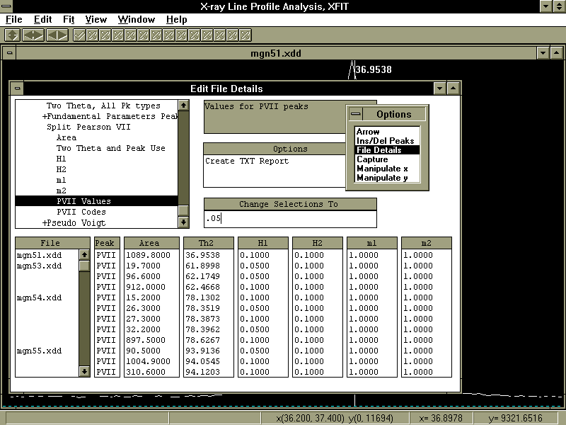
Figure 2. Display of the Edit File Details window.

1. Brief Instant Fitting Tutorials

XFIT has been designed to minimise user input with the use of defaults. These defaults can be altered as described in Appendix 5. The following are some brief getting started tutorials:

First run xfit.exe from within MS Windows.

Fitting two PVII peak to an MgO diffraction line.

i) Execute File/Load Data and load the example XRD file xfit_path\mgn51.xdd.

ii) LMB on Ins/Del Peaks in Options window.

iii) Change to PVII peak type in the Peak Edit Options window.

iv) LMB on the positions of the CuKa1 and the CuKa1 peaks.

v) Execute Fit/Fit Marqardt.

Fitting a PVII peak using an LAM

i) Execute File/Load Data and load the example XRD file xfit_path\mgn51.xdd.

ii) LMB on Ins/Del Peaks in Options window,

iii) Change to PVII peak type in the Peak Edit Options window.

iv) LMB on the position of the CuKa1 peak.

v) Assign the CUKA_2.LAM LAM file using Edit File Details/Assign LAMs to Files.

vi) Execute Fit/Fit Marqardt.

Assigning all of the parameters of one XRD file to another XRD file

i) Select the position Edit File Details/File/Path and Names of the XRD file name to be changed.

ii) Enter the new file name in the Change Selections To position and send it to the selected Edit File Details/File/Path and Names position.

1. Stripping ka2 from a Diffraction Line

XFIT offers a flexible means of stripping individual LAM lines from a calculated peak by setting the Use parameter of LAM lines to zero (see Appendix 1). The key-word no_normalize can be used to prevent XFIT from normalising the LAM profile.

1. Technical Details
2. Overview of Data Structures and Parameter Types

Table 4 shows a schematic of the data structures used by XFIT. All data and parameters assigned to an XRD is through graphical user input. Parameters are categorised as either XRD dependent (Background parameters for example) or Peak dependent (the integrated area under the peak for example). All data entered by the user can be saved to a project file (*.PRJ) which can be reloaded at a later time for continued analysis. XFIT loads LAMs from text files (see Appendix 2 for layout).

LAMs (no limit)

LAM

LAM lines (no limit)

XRD patterns (up to 32)

XRD pattern

XRD parameters

Background (up to 9th order orthogonalized Chebyshev polynomial)

LAM assigned

Peaks (no limit)

Peak

LAM assigned

Peak parameters

Table 4 The XRD and LAM data structures. Data types with "no limit" indicates no limit to the number of these data types.

1. Summary of Fundamental Parameters Approach

Important in the FP convolution approach is the ability to generate profile shapes with a modest amount of computational effort which has made it possible for its incorporation into XFIT. The physical parameters of the diffractometer of source length, sample length, slit length, receiving slit width, source width, horizontal divergence, and the primary and secondary Soller slits angles all become refinable parameters. Also refinable is specimen absorption, crystallite size and strain broadening.

FP includes the axial divergence aberration function for the general case of an X-ray diffractometer equipped with either a primary and/or secondary Soller slit configuration. This theoretical modelling of line profiles has been the subject of three research papers [2] [3] [4] and has invariably informed us at UTS of diffractometer mis-alignment and/or geometry irregularities.

1. Peak Types

Peak types and their corresponding peak dependent parameters are shown in table 5. Table 6 lists the generic unit area peak functions used for PV and PVII peaks.

Type	Name	Parameters assigned	Optional Parameters
Fundamental Parameters	FP	A, 2q	Strain (STR) and Crystallite Size (CS).
Pseudo-Voigt	PV	A, 2q, H,
Pearson VII	PVII	A, 2q, H1, H2, m1, m2

Table 5 Peak types and peak dependent parameters.

Unit area Gaussian	G = (g1/h) exp(g2 x2 / h2)	where g1 = 2 (ln(2) / )½ and g2 = -4 ln(2)
Unit area Lorentzian	L = (l1/h) / (1+l2 x2/h2)	where l1 = 2 / and l2 = 4
Unit area PV	PV = ( L + (1-) G)	where h = FWHM
Unit area PVII	PVII = [ (1 + b1 x2)-m1 + (1 + b2 x2)-m2] / a where a = ½ (½) [ (m1-½) / ((m1) b1½) + (m2-½) / ((m2) b2½) ] b1 = 4 (21/m1 - 1) / and b2 = 4 (21/m2 - 1) /

Table 6 Generic unit area peak functions.

1. Generation of a Peak

Peaks are generated starting with an LAM, the actual LAM used for generation is determined as follows:

XFIT uses the LAM assigned to the peak, otherwise

XFIT uses the LAM assigned to the XRD, otherwise

XFIT uses a default LAM consisting of one LAM line as described in Appendix 2.

The type of LAM lines generated depends on the peak type and can be either PV, PVII or FP type lines. The next stage of peak generation convolutes the generated LAM with assigned specimen or instrumental type aberrations, as shown in equation (1),

(1)

where A is the area under the peak and SW, CS and LOR are convolutions described in section 4.6. For FP type peaks the SW, CS and LOR convolutions are performed analytically. All other convolutions are performed numerically including SW, CS and LOR for non-FP peaks.

1. Preliminary to Refinement

An LAM file determines the number of emission profile lines generated for a peak. Table 7 shows the typical data contained within an LAM file. Eo,i, Eh,i and EA,i are parameter names used to identify the LAM data.

Table 7 Relative intensities, wavelengths and lifetime widths of the Cu Ka spectrum taken from Berger [1] with the wavelengths scaled to make the peak wavelength for CuKa1 = 1.5405981Å.

Emission Line Satellites K1a K1b K2a K2b

Eo,i Eh,i EA,i Relative (Å) (Å x 10-3) Intensity 1.534753 3.69 0.0160 1.540596 0.44 0.5692 1.541058 0.60 0.0762 1.544410 0.52 0.2517 1.544721 0.62 0.0871

The interpretation of the LAM data is dependent on the peak types. Eo,r, Eh,r and EA,r correspond to the emission line with the largest EA,i value. It is used to calculate the d spacing for the peak .

The relative areas under an emission line are determined by EA,i. The peak parameter A of equation (1) determines the total area under all of the emission lines for that peak. Before scaling by the A parameter, the area under all of the emission lines is scaled to unity.

For all peak types the position of a particular emission line 2qi in terms of the peak parameter 2q is determined by the following:

2 d = Eo,r / sin(q)

Eo,i = 2 d sin(qi) = (Eo,r / sin(q)) sin(q + qi)

or 2qi = ((Eo,i / Eo,r) - 1) (tan(q) 360 / )

or 2qi = 2q + 2qi

The half-width parameter(s) in 2q for an emission line i are determined by the relations shown in table 8:

Table 8. Half-widths in 2q for an emission line i.

FP PV PVII

Half-width in 2q Hi = (h,i / o,r )(tan(q) 180 / ) Hi = H Eh,i / Eh,r H1,i = H1 Eh,i / Eh,r H2,i = H2 Eh,i / Eh,r

1. Parameter Types and Aberration Functions

All parameters in table 9 represent an aberration function that, if selected, will be convoluted into the peak as described in equation (1). The parameters of table 10 represent the full axial divergence aberration function as described in [4]. The independent angular variable e, in terms of the measured angle 2 and the Bragg angle 2q , is defined by.

Table 9 Instrumental, specimen and miscellaneous convolutions.

Full axial divergence aberration function parameters.
Receiving Slit Length	SL (mm)	Length of receiving slit.
Sample Length	SAML (mm)	Length of sample.
Source Length	SOUL (mm)	Length of source.
Primary Soller Angle	PS ()	Angle transmitted by the primary Soller slits. Includes a Use attribute.
Secondary Soller Angle	SS ()	Angle transmitted by the secondary Soller slits. Includes a Use attribute.

Table 10 The five parameters used to describe the full axial divergence aberration function with either primary and/or secondary Soller slits.

1. The Convolution Step Parameter

The XRD dependent Convolution Step integer, found in the Edit File Details window, corresponds to the number of calculated data points per measurement data point used to calculate the calculated pattern. It is useful when numerical instabilities are introduced. This can happen when a particular convolution has a small effect on the profile shape or when the measurement step is large.

1. Parameter Attributes

Parameters are assigned the five attributes shown in table 11. These are sometimes hidden from the user as in the case of the Use parameters for the axial divergence parameters of table 10. In that case a single Use parameter signals the use of the three axial divergence length parameters.

Use	Boolean switch to indicate the use of the parameter in the calculated pattern.
Code	A string parameter which, when the first character is not '0', indicates to the refinement procedure that this parameter is to be refined. When the first character is '@' the refinement procedure treats the parameter independently (not related to any other parameter) during refinement.
Constraint	See text and equation (2).
Value	The parameters value.
Error	The parameters error.

Table 11 The five parameters used to describe the axial divergence aberration function parameters with primary and secondary Soller slits.

Constraints are an important aspect of refinement that allow groups of parameters to be algebraically related during refinement. For example, two peaks from the same phase with expected similar crystallite size (CS) should have a single CS parameter assigned. This is accomplished by constraining the individual CS's to the same value when the peaks are refined simultaneously. More generally, the algebraic relationship between n parameters are written in terms of a reference parameter Pr such that:

or, Pi + c Pr = constant

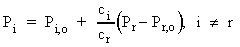
(2)

where Pi and Pi,o represent a parameter at the end of an iteration and at the start of the refinement process respectively, the ci and cr constants define the relationship between Pi and Pr. The refinement procedure then considers only one parameter Pr where the derivative of the calculated patterns Yc with respect to Pr becomes

(3)

Every relationship between two parameters that can be written in the form of (2) reduces by one the number of parameters in the refinement procedure. By doing this, physically meaningful relationships are maintained and instabilities due to parameter correlation eliminated. XFIT implements the constraints of equations (2) through the Code attribute. Codes that are identical for similar parameter types invokes the constraining relationship of equation (2). For example, to constrain the CS's of two peaks to the same value, a code of cs could be given to both the CS parameters. If the same Code was given to two parameters that are not of the same type, eg. FS and CS, then the refinement procedure would not apply the constraining equation of (2). To constrain parameters that are not of similar type, eg. H1 and H2 of PVII peaks, then start the Code attribute with the character '*'.

1. Calculating Peak 2 Limits

The minimum and maximum 2 limits for calculated peaks are mainly handled internally by XFIT. Peaks with convolution parameters assigned has their 2 limits extended as required during convolution calculations. XFIT does allow, through the LAM file, limits to be set for the FP LAM lines as described in Appendix 2.

The limits for PVII LAM lines are calculated such that the maximum/minimum y ratio, (ymax/yn) of equation (4), is 500 for both y1 and y2, or ymax/y1 = ymax/y2 = 500.

., where bn is as defined in table 6.

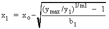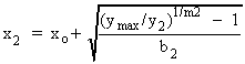
(4)

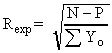
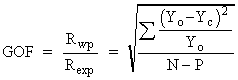
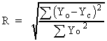
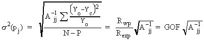
Appendix 1. Profile Agreement Indicators

The Edit File Details window contains the following global and XRD dependent profile Agreement Indicators:

,

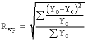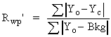Appendix 2. Example LAM File

/* Block and nested block comments are allowed. */

' text from this character to the end of the line is a comment.

/*

Example CuKa Emission Profile - File Details.

Format of an emission line :

lam Use

la Value Code Constraint Error

lo Value Code Constraint Error

lh Value Code Constraint Error

where

la Value = Relative area under the emission line.

lo Value = Wavelength of the emission line (Å).

lh Value = Lifetime widths (Å x 10-3).

The order of la, lo and lh is not important but they do all have to exits.

The Code attribute is used for refinement as described in section 4.7.

A single Use parameter is used to determine use of each emission line.

*/

no_normalize

lam 1 la 0.015885 0 1 0 lo 1.534753 0 1 0 lh 3.68545 0 1 0 num_hw 6

lam 1 la 0.076152 0 1 0 lo 1.541058 0 1 0 lh 0.60000 0 1 0 num_hw 10

lam 1 la 0.251690 0 1 0 lo 1.544410 0 1 0 lh 0.52000 0 1 0 num_hw 10

lam 1 la 0.569208 0 1 0 lo 1.540596 0 1 0 lh 0.43700 0 1 0 num_hw 10

lam 1 la 0.087065 0 1 0 lo 1.544721 0 1 0 lh 0.62000 0 1 0 num_hw 10

/*

The num_hw (optional) = number of lorentzian FWHMs to include in the calculation of the LAM line when the peak type if FP.

The no_normalize key-word informs XFIT not to normalize the area under the LAM to unity.

*/

/*

THE DEFAULT LAM

================

The following default LAM line is used when a peak has no LAM file assigned:

lam 1 la 1 0 1 0 lo 1 0 1 0 lh 1 0 1 0

*/

Appendix 3. File Types and Formats

The XRD data files read by XFIT are all ASCII text files. Their formats are shown in table 12. Comments can appear in any of the files and are of the following form:

/* Block and nested block comments are allowed. */

' text from this character to the end of the line is a comment.

Other file extensions that has the *.XDD format that can be read by XFIT are:

*.BKG, *.CPT, *.CAL, *.LN, *.DIF, *.PK

File Type	Format	Explanation
*.XDD	line comment	An optional line at the start of the file
	start angle	start angle of XRD pattern.
	step angle	step angle of XRD pattern.
	finish angle	finish angle of XRD pattern.
	counting time	time spent counting at measured steps.
	an unused number	Not used by XFIT
	wavelength (Å)	Not used by XFIT
	I1 I2 I3 etc.......	Observed XRD data points. Data separators can be space(s), tabs or new-line character (i.e. white space characters).
*.XY	x1 y1 x2 y2 x3 y3 etc.........	Two columns of numbers corresponding to the x and y data values. Data separators can be space(s), tabs or the new-line character (i.e. white space characters).
*.CPI	line comment	must exist.
	start angle	start angle of XRD pattern.
	finish angle	finish angle of XRD pattern.
	step angle	step angle of XRD pattern.
	anything ....
	SCANDATA	Key-word before the start of the observed data.
	I1 I2 I3 etc.......	Observed XRD data points. Data separators can be space(s), tabs or new-line character (i.e. white space characters).

Table 12 File formats read by XFIT.

Appendix 4 The Non-Linear Least Squares Routine

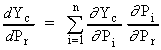
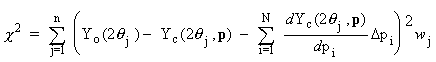
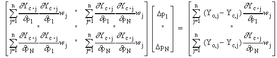
The non-linear least squares routine used by XFIT is based on the Newton-Raphson method. Here the diffraction pattern Yc is calculated as a function of 2qj. It is expanded to a first order Taylor series around the parameter vector p ignoring second order terms. Yc in terms of N parameters and n diffraction points (j = 1, n) become:

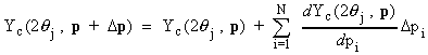(5)

where the parameters pi (i = 1 to N) are assumed to be the actual values being fitted. The function 2 is then minimised iteratively with respect to the pi's to obtain the best fit to the observed data Yo(2qj) and is given by

(6)

where the weighting function wj=1/j2 and j is the standard error in the data point j. To minimise equation (6), partial derivatives with respect to the pi's are equated to zero:

, or

or in matrix form

This represents a linear set of equations in pi's. These are solved using matrix methods for each iteration of the refinement. Parameters are updated at the end of each iteration with values corresponding to pi + pi.

A number of additional features have been incorporated in the present non-linear least squares routine. These include the use of the robust Marquardt method [5], and the powerful Singular Value Decomposition (SVD) method [6] for solving the matrix equation A p = b. SVD allows singular or ill-conditioned A matrices to be processed such that instabilities are identified whilst the residual A p ­ b is being minimised. It has been of great benefit in this analysis.

Appendix 5 The design of XFIT and Setting Parameter Defaults

On execution, XFIT loads the text file temdoc8.cpp that basically controls its behaviour. By changing temdoc8.cpp, it is possible to considerably modify the behaviour of XFIT without re-compiling. temdoc8.cpp also contain the defaults for all parameters. These are found by editing/searching for prm_defaults. Under this heading the various parameters are easily recognised. An example of the Slit Length defaults is shown in table 13. These are all optional and can be changed as required. The order of appearance of the default types is not important.

Default type	Value
min	0.001	The minimum allowed value for the Value attribute.
max	50.0	The maximum allowed value for the Value attribute.
use	0	The Use attribute.
code	0	The Code attribute.
val	12.0	The Value attribute.
fmt_val	%-1.3f	The c type format for the Value attribute.
fmt_err	%-1.2f	The c type format for the Error attribute.

Table 13. Example defaults for the Slit Length parameter.

References

1. Berger, H. (1986). X-ray Spectrometry 15, 241-243.

2. Cheary, R. W. & Coelho, A. A. (1992). "A Fundamental Parameters Approach of X-ray Line-Profile Fitting". J Appl. Cryst. 25, 109 - 121.

3. Cheary, R. W. & Coelho, A. A. (1994). "Synthesising and Fitting Linear Position-Sensitive Detector Step-Scanned Line Profiles". J Appl. Cryst. 27, 673 - 681.

4. Cheary, R. W. & Coelho, A. A. (1996). "Theoretical Model for Axial Divergence with Primary and Secondary Soller Slits in X-ray Line-Profile Analysis". In preparation.

5. Marquardt, D. W. (1963). J. Soc. Ind. Appl. Math., vol 11, pp 431-331

6. Nash, J. C. (1990). Compact Numerical Methods for Computers, Adam Hilger, Bristol and New York.